0%

皮尔森(逊)相关系数(Pearson Correlation Coefficient, PCC)

摘要

\(R\) :相关系数(correlation coefficient),即皮尔森相关系数,值位于 -1 到 1 之间,即负相关和正相关,绝对值越大表明相关性越强,P值越小越相关。

\(R^2\) :决定系数(coefficient of determination),\(R^2\) 值越接近 1,吻合程度越高,越接近 0,则吻合程度越低。

决定系数 = 相关系数平方

皮尔森相关系数

皮尔森相关系数也称皮尔森积矩相关系数(Pearson product-moment correlation coefficient) ,是一种线性相关系数,是最常用的一种相关系数。记为 R,用来反映变量X和变量Y的线性相关程度,R 值介于-1到1之间,绝对值越大表明相关性越强。[1]

适用连续变量。

相关系数 与相关程度一般划分为

  • 0.8 - 1.0 极强相关

  • 0.6 - 0.8 强相关

  • 0.4 - 0.6 中等程度相关

  • 0.2 - 0.4 弱相关

  • 0.0 - 0.2 极弱相关或无相关

原假设:两者不存在相关性 P值小,即我们观察的样本(不存在相关性)发生的概率小,存在相关性的概率大,如果原假设成立即不存在相关性,那么我们这个样本就很极端很显著。

相关系数绝对值越大,越相关,P值越小越相关。

scipy.stats.pearsonr(x, y, *, alternative='two-sided')[2]

1
2
3
4
5
6
7
8
9
10
11
12
# Python实现
from scipy.stats import pearsonr

x = [1,2,3,4]
y = [1.2,2.2,3.1,4.1]
result = pearsonr(x,y)
print("pearson相关系数: {:.6f}".format(result.statistic)) # result[0]
print("P-Value: {:.6f}".format(result.pvalue)) # result[1]

# out:
# pearson相关系数: 0.999783
# P-Value: 0.000217

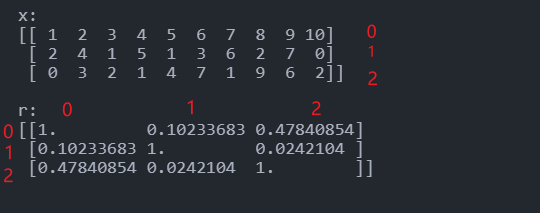
numpy.corrcoef(x, y=None, rowvar=True, bias=<no value>, ddof=<no value>, *, dtype=None)

Return Pearson product-moment correlation coefficients.[5]

这里计算的是特征与特征(行与行/列与列)的相关系数。
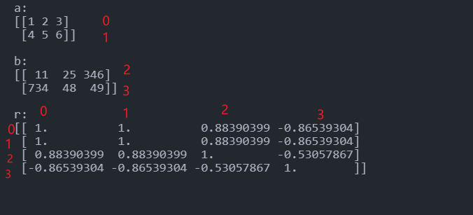
1
2
3
4
5
6
7
8
9
10
11
12
13
14
15
16
17
18
19
import numpy as np
a = pd.Series([1,2,3,4,5,6,7,8,9,10])
b = pd.Series([2,4,1,5,1,3,6,2,7,0])
c = pd.Series([0,3,2,1,4,7,1,9,6,2])
x = np.vstack((a,b,c))
r = np.corrcoef(x)
print("x:\n{}\n".format(x))
print("r:\n{}".format(r))

# out:
# x:
# [[ 1 2 3 4 5 6 7 8 9 10]
# [ 2 4 1 5 1 3 6 2 7 0]
# [ 0 3 2 1 4 7 1 9 6 2]]

# r:
# [[1. 0.10233683 0.47840854]
# [0.10233683 1. 0.0242104 ]
# [0.47840854 0.0242104 1. ]]

1
2
3
4
5
6
7
8
9
10
11
12
13
14
15
16
17
18
19
20
21
22
a = np.array([[1, 2, 3], [4, 5, 6]])
b = np.array([[11, 25, 346], [734, 48, 49]])
r = np.corrcoef(a,b)

print("a:\n{}\n".format(a))
print("b:\n{}\n".format(b))
print("r:\n{}\n".format(r))

# out:
# a:
# [[1 2 3]
# [4 5 6]]

# b:
# [[ 11 25 346]
# [734 48 49]]

# r:
# [[ 1. 1. 0.88390399 -0.86539304]
# [ 1. 1. 0.88390399 -0.86539304]
# [ 0.88390399 0.88390399 1. -0.53057867]
# [-0.86539304 -0.86539304 -0.53057867 1. ]]

线性回归的R平方

线性回归后得到的 R 平方和使用皮尔森相关求得的 R 再平方数值上面是一样的。[3]

R平方:决定系数,反应因变量的全部变异能通过回归关系被自变量解释的比例。\(R^2\) 值越接近1,吻合程度越高,越接近0,则吻合程度越低。\(R^2\) 作为相关系数,一般机器默认的是\(R^2\) >0.99,这样才具有可行度和线性关系。[4]

参考文献

+