快速查询:Python 函数的简单解释及使用
了解任何函数的最佳方式,谷歌搜索,找到函数的官方文档,阅读。
详细可参考:搜索使用
常用包下载
1
2
3
4
5
6
7
| pip install numpy
pip install pandas
pip install scikit-learn
pip install matplotlib
pip install tqdm
pip install seaborn
|
excel
导入 excel
1
2
3
4
5
6
7
8
9
10
11
12
13
14
| import pandas as pd
excel_path = r'D:\MyData\Boston_data.xlsx'
df = pd.read_excel(excel_path, sheet_name='page_1')
print(df)
with pd.ExcelFile(r"D:\MyData\数据.xlsx") as xls:
df1 = pd.read_excel(xls, "page1")
df2 = pd.read_excel(xls, "page2")
df3 = pd.read_excel(xls, "page3")
|
导出 excel
array导出为excel:
1
2
3
4
5
6
7
8
9
10
|
import pandas as pd
data_df = pd.DataFrame(data)
target_df = pd.DataFrame(target)
Boston_all = pd.concat([data_df,target_df],axis=1)
excel_path = r'D:\MyData\Boston_data.xlsx'
with pd.ExcelWriter(excel_path) as writer:
Boston_all.to_excel(writer, 'page_1')
|
numpy
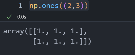
np.one()
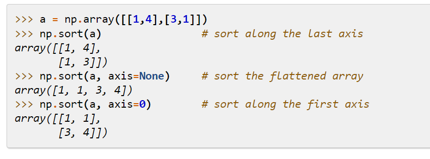
np.sort()
sort()
给数组元素排序, 返回也是数组array
np.argsort()
np.argsort()
1
2
3
| x = np.array([3, 1, 2])
np.argsort(x)
array([1, 2, 0])
|
pandas
pd.concat()
concat()
对dataframe或者series进行拼接
pd.concat([df1,df2],axis=0):
0为index方向即上下方向,1为index方向即左右方向
1
2
3
4
5
6
| df1 = pd.DataFrame(data=np.ones((3,3))*1,columns=["a","b","c"],index=[0,1,2])
df2 = pd.DataFrame(data=np.ones((3,3))*2,columns=["a","b","c"],index=[0,1,2])
df3 = pd.DataFrame(data=np.ones((3,3))*3,columns=["d","e","f"],index=[0,1,2])
print(df1)
print(df2)
print(df3)
|
1
2
3
4
5
6
7
8
9
10
11
12
| a b c
0 1.0 1.0 1.0
1 1.0 1.0 1.0
2 1.0 1.0 1.0
a b c
0 2.0 2.0 2.0
1 2.0 2.0 2.0
2 2.0 2.0 2.0
d e f
0 3.0 3.0 3.0
1 3.0 3.0 3.0
2 3.0 3.0 3.0
|
1
| pd.concat([df1,df2],axis=0)
|
1
2
3
4
5
6
7
| a b c
0 1.0 1.0 1.0
1 1.0 1.0 1.0
2 1.0 1.0 1.0
0 2.0 2.0 2.0
1 2.0 2.0 2.0
2 2.0 2.0 2.0
|
1
| pd.concat([df1,df2],axis=1)
|
1
2
3
4
| a b c a b c
0 1.0 1.0 1.0 2.0 2.0 2.0
1 1.0 1.0 1.0 2.0 2.0 2.0
2 1.0 1.0 1.0 2.0 2.0 2.0
|
zip
将对象中对应的元素打包成一个个元组,然后返回由这些元组组成的列表。在
Python 3.x 中为了减少内存,zip() 返回的是一个对象。如需展示列表,需手动
list() 转换。
语法:
1
2
| zip([iterable, ...])
# iterable -- 一个或多个迭代器(列表等);
|
1
2
3
4
5
6
7
8
9
| >>> a = [1,2,3]
>>> b = [4,5,6]
>>> c = [4,5,6,7,8]
>>> zipped = zip(a,b)
>>> zipped
<zip object at 0x103abc288>
>>> list(zipped)
[(1, 4), (2, 5), (3, 6)]
|
解压:星号
1
2
3
4
5
6
| >>> a1, a2 = zip(*zip(a,b))
>>> list(a1)
[1, 2, 3]
>>> list(a2)
[4, 5, 6]
>>>
|
1
2
3
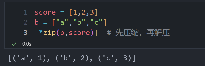
| score = [1,2,3]
b = ["a","b","c"]
[*zip(b,score)]
|
df.columns
获得dataframe的列索引即列名,可将其转换为列表:df.columns.tolist()
Machine learning
划分训练集,验证集,测试集
训练集就像是学生的课本,学生
根据课本里的内容来掌握知识,验证集就像是作业,通过作业可以知道
不同学生学习情况、进步的速度快慢,而最终的测试集就像是考试,考的题是平常都没有见过,考察学生举一反三的能力。
- 训练集(Training Dataset):训练阶段使用
- 验证集(Validation
Dataset):调整超参数(在机器学习模型中,需要人工选择的参数称为超参数。超参数选择不恰当,就会出现欠拟合或者过拟合的问题。),让模型处于最好状态。没有超参数可以不使用验证集,可直接用测试集评估效果。
- 测试集(Test Dataset):评估模型
1
2
| from sklearn.model_selection import train_test_split
X_train,X_test,y_train,y_test = train_test_split(X,y,test_size = 0.2,random_state=0)
|
将特征数据存储在 X 中,目标数据存储在 y 中。test size
参数指定了测试集占整个数据集的比例,这里设置为0.2表示测试集占20%。random
state 参数用于设置随机种子,以确保每次划分得到相同的结果。
1
2
3
| from sklearn.model_selection import train_test_split
X_train,X_valtest,y_train,y_valtest = train_test_split(X,y,test_size = 0.4,random_state=0)
X_val,X_test,y_val,y_test = train_test_split(X_valtest,y_valtest,test_size = 0.5,random_state=0)
|
参数网格寻优
选择超参数(需要人工选择的参数称为超参数)的时候,有两个途径,一个是凭经验微调,另一个就是选择不同大小的参数,带入模型中,挑选表现最好的参数。使用Scikit-Learn的GridSearchCV来做这项穷举参数,搜索最好表现的参数组合工作。
GridSearchCV的名字其实可以拆分为两部分,GridSearch和CV,即网格搜索和交叉验证[1]。网格搜索,搜索的是参数,即在指定的参数范围内,按步长依次调整参数,利用调整的参数训练学习器,从所有的参数中找到在验证集上精度最高的参数,这其实是一个训练和比较的过程。交叉验证保证模型正确反映数据的真实情况,减少误差。
本质上就是穷尽参数,找出表现最好的一组参数,所以输入就需要:
1、用什么模型 2、可选参数(不同算法模型,参数不一样) 3、几折交叉
输出就是: 1、最好的参数组合 2、最好的模型
GridSearchCV
官方文档
1
2
3
4
5
6
7
| clf = KNeighborsClassifier()
parameters = {'n_neighbors': [i for i in range(1,10)]}
gc = GridSearchCV(clf, parameters, cv=5)
gc.fit(X_val, y_val)
best_p = gc.best_params_
bestknn = gc.best_estimator_
test_score = bestknn.score(X_test,y_test)
|
k 折交叉验证
1
2
3
| from sklearn.model_selection import cross_val_score
scores = cross_val_score(Logreg,iris.data,iris.target,cv=5)
print("Average cross-validation score:{:.2f}".format(scores.mean()))
|
KNN (k近邻)
1
2
3
4
5
6
7
8
9
10
11
12
13
|
from sklearn.neighbors import KNeighborsClassifier
knn = KNeighborsClassifier(n_neighbors=1)
knn.fit(X_train, y_train)
prediction = knn.predict(X_test)
score = knn.score(X_test,y_test)
from sklearn.neighbors import KNeighborsRegressor
knn = KNeighborsRegressor(n_neighbors=1)
knn.fit(X_train, y_train)
prediction = knn.predict(X_test)
score = knn.score(X_test,y_test)
|
SVM
核支持向量机(kernelized support vector
machine),通常简称为SVM。
- 在低维数据和高维数据表现都很好(少特征和多特征)
- 1万样本可能还好,10万样本运行内存和时间面临挑战
- 预处理和调参要非常小心,与随机森林和梯度提升则相反(很少预处理,甚至不需要)
1
2
3
4
5
6
7
8
9
10
11
12
13
14
| from sklearn.svm import SVR
svr_rbf = SVR(kernel="rbf", C=100, gamma=0.1, epsilon=0.1)
svr_lin = SVR(kernel="linear", C=100, gamma="auto")
svr_poly = SVR(kernel="poly", C=100, gamma="auto", degree=3, epsilon=0.1, coef0=1)
svr_rbf.fit(X_train, y_train)
prediction = svr_rbf.predict(X_test)
score = svr_rbf.score(X_test,y_test)
|
RF
参考文章